04. Two DoF Arm
Two Degrees of Freedom
Building a two-degree-of-freedom serial manipulator
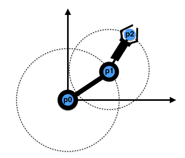
You've now seen how a system of two points can be constrained down to just one degree of freedom (DoF) by connecting the points with a rod and anchoring the system at one end. Now, let's add a third point and a second DoF to build a robotic arm! Our system now looks like the image above, where p0 is the base of the two-link arm.
Constraints on a 2-DoF serial manipulator
SOLUTION:
The position of p0 and the length of the links connecting p0 to p1 and p1 to p2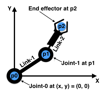
Here is our 2-DoF manipulator with all the parts labeled. Let's assume the base (Joint-0) is fixed at the origin (0, 0) of our coordinate system.
Additional parameters
SOLUTION:
The angle of Link-1 away from the x-axis and the angle of Link-2 from the Link-1 axisCoding it up:
Now it's time to code up the 2-DoF arm! This will be a test of your intuition (and knowledge of trigonometry). Let's assume the position of the base of the arm (p0 above) is located at the origin (0, 0). Then once you have the length of the two links, all you need are the angles of the joints to completely specify the configuration of the arm.
In the quiz below, your job is to write a function that takes as inputs the length of each of the two links, and the joint angles, and outputs the (x, y) position of the joint at p1 and the end effector at p2. So it will look like this:
# Define a function to compute the arm configuration
# NOTE: joint1_angle is the angle counterclockwise from the link1 axis
def compute_arm_config(link1_length, link2_length, joint0_angle, joint1_angle):
    # TODO: compute the (x, y) position of the p1 joint and the end effector at p2.
    #  joint1_x =
    #  joint1_y =
    #  p2_x =
    #  p2_y =
    return joint1_x, joint1_y, p2_x, p2_y
When you succeed you will have solved the forward kinematics problem for a 2-DoF arm on a plane!
Start Quiz:
Proof
Still struggling to solve this system? if yes, we will draw the free-body diagram of this system and work out the steps leading toward the solution. Before you start, take a look at the Trigonometry with right triangles tutorials to refresh your math skills.
](img/untitled-presentation-1.png)
At the local frame 1, solving the position of P1 with respect to the global frame at P0:
At the local frame 2, solving the position of P2 with respect to the reference frame at P1:
Finally, putting it all together and solving the position of the end effector P2 with respect to the global frame at P0: